Residual flows [1, 2] are a special class of normalizing flows whose building blocks are residual layers of the form $ x \to x + g_\theta(x) $. In this post, we’ll discuss the math behind residual flows, how they’re implemented in practice, and their connection to flow-based generative models.

Background: Normalizing Flows

A common problem in generative modeling is as follows: given a Gaussian source distribution $p_0$ and target distribution $p_1$, we wish to learn an invertible, bijective transformation $F_\theta$ which maps $p_0$ to $p_1$. Examples of $p_1$ inclue Gaussians, and distributions over images, molecular conformations, pine trees in Finnish forests, etc. (Discrete) normalizing flows parameterize $F_\theta$ as the composition $F_\theta = F^N_\theta \circ \dots \circ F^i_\theta$, from which $\log p_1(F_\theta(x))$ can be computed using the change of variables formula

\[\log p_0(x) = \log p^\theta_1(F_\theta(x)) + \log \left\lvert \det \frac{\partial F_\theta(x)}{\partial x}\right\rvert = \log p^\theta_1(F_\theta(x)) + \sum_{k=1}^N \log \left\lvert \det \frac{\partial F_\theta^k(x)}{\partial x}\right\rvert,\]

where $\det \frac{\partial F_\theta(x)}{\partial x}$ denotes the Jacobian and $p^\theta_1$ is the approximation of $p_1$ given by $F_\theta$. Provided that the change of variables formula is tractable, normalizing flows can then be trained using maximum likelihood. Significant effort has been dedicated to developing expressive, invertible building blocks $F_\theta^i$ whose Jacobians have tractable log-determinant. Successful approaches include coupling-based, autoregressive, and spline-based flow architectures. For a more detailed introduction to discrete normalizing flows, see Lilian Weng’s blogpost here.

As it turns out, we can also (and in fact it is productive to so) parameterize the map $F_\theta$ as the pushforward of $p_0(x)$ by the “flow” of a time-dependent vector field $u_\theta(x,t)$. In this case, there is a continuous change of variables formula given by

\[\log p_0(x) = \log p^\theta_1(x) - \int_0^1 \text{Tr}\left(\frac{\partial F_\theta(x)}{\partial x}\right)\, dt.\]

Such a parameterization via $u_\theta(x,t)$ is known as a continuous normalizing flow, and was introduced first as a neural ode, and then improved in FFJORD via the Hutchinson trace estimator, which we will discuss at length later on.

Background: Lipschitz Continuity, Spectral Norm, and Power Iteration

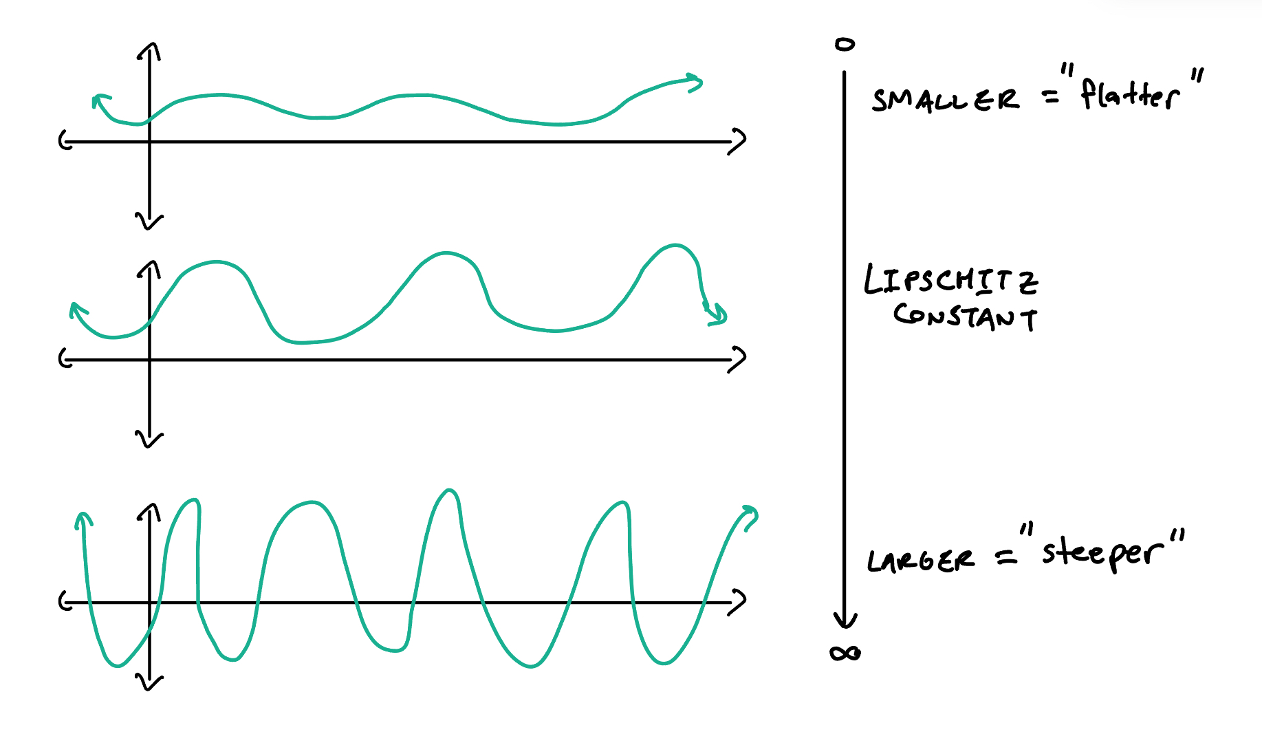
There are a few ideas to touch on before we can actually talk about residual flows. The first is the idea of Lipschitz continuity. Basically, a function $f: \mathbb{R} \to \mathbb{R}$ is Lipschitz continuous if there’s an upper bound on how fast $f$ changes value. In other words, there’s some constant $K$ so that $|f(x) - f(y)| \le K|x - y|$ is always true. The smallest such value of $K$ is said to be the Lipschitz constant of $f$, and is denoted $\text{Lip}(f)$.

Lipschitz continuous functions with successively higher Lipschitz constants. The steeper the function, the higher the Lipschitz constant.

Of course, we can generalize this idea, and since we’ll be thinking about vectors, the definition we’ll be using involves a function $f: \mathbb{R}^d \to \mathbb{R}^d$ which is Lipschitz continuous iff there exists $K$ so that \(\lVert f(x) - f(y) \rVert_2 \le K \lVert x-y \rVert_2\). We can now state the useful Banach fixed point theorem.

Moving on, suppose that $f$ is linear, and because it’s linear, let’s call it $T$ instead. We care about the linear case because we’ll eventually be thinking about neural networks which contain linear layers. What has to be true about $T$ for it to be Lipschitz continuous, and if it is, what is the Lipschitz constant? Writing down the inequality \(\lVert T(x) - T(y) \rVert_2 \le K \lVert x-y \rVert_2\), and using the fact that since $T$ is linear, $T(x) - T(y) = T(x-y)$, we see that for any such $x,y$, $\lVert T(x-y) \rVert \le K\lVert x-y \rVert $. Writing $z \triangleq x - y$, we find that for any such $z$, $\lVert Tz \rVert \le K \lVert z \rVert$. Thus, $K$ must simply satisfy $K \le \lVert T \rVert_2 \triangleq \inf_z \frac{\lVert Tz \rVert_2}{\lVert z \rVert_2}$. This value $\lVert T \rVert_2$ is known as the spectral norm of $T$.

As it turns out, the spectral norm of a matrix is equal to its largest singular value $\sigma_1$ (singular values generalize eigenvalues to non-square matrices), which can be computed using a technique called power iteration. The idea is to initialize $x_0$ arbitrarily, and to generate \(\{ x_n \}_{n=1}^\infty\) by $x_n \triangleq \frac{Tx_{n-1}}{\lVert Tx_{n-1} \rVert_2}$ (in other words, the normalized “orbit” of $x_0$). If the projection of $x_0$ onto the right singular vector (think: eigenvector, but for non-square matrix) is non-zero, then the Rayleigh quotients will converge to the square of the largest singular value $\sigma_1$. When we cannot guarantee the non-zero projection constraint, we can only say that the Rayleigh quotients converge to some lower bound on $\sigma_1$.

Residual Flows as Normalizing Flows

With residual flows, the idea is to parameterize our normalizing flow map as $F_\theta = F_\theta^1 \circ \dots \circ F_\theta^N$, where each layer is of the form $F_\theta^i: x \to x + g_i^\theta(x)$ and where $g_\theta(x)$ is Lipschitz continuous with Lipschitz constant less than one. This Lipschitz constraint, and the proposed implementation, is the big idea here which allows the residual form of the $F_\theta^i$ to function as a normalizing flow.

Invertibility. To see that $F_\theta$ is invertible, it suffices to show that $F^i_{\theta}: x \to x + g^i_\theta(x)$ is invertible for each $i$. Let $y \in \mathbb{R}^d$. Then we would like to show that there exists a unique $x \in \mathbb{R}^d$ satisfying $y = F^i_{\theta}(x) = x + g^i_\theta(x)$. Then $x$ is a fixed point of the map $h: x \to y - g^i_\theta(x)$. Note that since $g^i_\theta(x)$ is Lipschitz continuous with constant $K < 1$, $h$ is also Lipschitz continuous with Lipschitz constant $\tilde{K} = K < 1$. Thus, the Banach fixed point theorem guarantees that $h$ has a unique fixed point, and in turn that a unique $x$ exists. As $y$ was arbitrary, we conlude that each of the $F_\theta^i$, and thus $F$ as well, are invertible.

Tractable Log-Det-Jac. The change of variables formula says that \[\log p_0(x) = \log p_1(x) + \log \left\lvert \det \frac{\partial F_\theta^i(x)}{\partial x}\right\rvert \] where $p_0$ where \(p_1 \triangleq {[F_\theta^i]}_\sharp (p_0)\) is the pushforward of $p_0$ by $F_\theta^i$. Intuitively, the application of $F_\theta^i$ will stretch and squish the distribution of initial distribution $p_0$ of $x$’s, giving $p_1$. The change of variables formula makes this squish factor precise. Thus, it’s important that we know how to evaluate the logarithm of the absolute value of the determinant of the Jacobian (log-det-Jac) \(\frac{\partial F_\theta^i(x)}{\partial x}\). The thing to do is to observe that \[ \begin{aligned} \log \left\lvert \det \frac{\partial F_\theta^i(x)}{\partial x}\right\rvert = \log \left\lvert \det \frac{\partial}{\partial x}\left(x + g_\theta^i(x)\right)\right\rvert = \log \left\lvert \det \left(I + \frac{\partial g_\theta^i(x)}{\partial x}\right)\right\rvert = \text{Tr}\log \left(I + \frac{\partial g_\theta^i(x)}{\partial x}\right). \end{aligned} \] Here, the use of $\log$ on the right-most side denotes the matrix-logarithm (the inverse of the exponential map). Writing \(J_g(x) \triangleq \frac{\partial g_\theta^i(x)}{\partial x}\) (dropping the subscript for brevity), we can expand the RHS as a power series via \[ \text{Tr}\log \left(I + J_g(x)\right) = \text{Tr} \left(\sum_{k=0}^\infty \frac{(-1)^k}{k}J_g(x)^k\right). \] The only problem now is that this is an infinite series, so we cannot possibly evaluate it completely in its current form. The authors of i-ResNet ([1]) propose to do the following:

1. Pick some reasonable $N$ and truncate the series after $N$ terms.
2. Estimate the trace of the resulting truncated series using the unbiased Hutchinson trace estimator (see below).

The issue with truncation is that the terms decay exponentially in the Lipschitz constant of $g_\theta^i$ (this follows from the fact that $\lVert J_g(x)^k \rVert_2 \le K^k$), so that the closer $K$ is to one, the slower the convergence of the series is. There is therefore a tradeoff between the accuracy or bias incurred by the truncation, and the computation neeed.

The Hutchinson Trace Estimator

Once we have chosen some value of $N$ to truncate the series at, it is still computationally expensive to compute the trace

\[ \text{Tr} \left(\sum_{k=0}^N \frac{(-1)^k}{k}J_g(x)^k\right). \] Why is this difficult? Consider the simpler problem of computing $\text{Tr} (J_g(x))$. Since $J_g(x) = \frac{\partial g_\theta^i(x)}{\partial x}$, the trace $\text{Tr} (J_g(x))$ is given by the sum \(\sum_i \frac{\partial g(x)_i}{x_i}\). This requires $d$ (the dimensionality of $x$) separate backward passes through autograd which is expensive. It gets even worse because our actual summation involves $N + 1$ such terms. The fact that the other terms $J_g(x)^k$ are powers of the Jacobian fortunately does not complicate the situation too much: since the product of Jacobians corresponsds to the Jacobian of the composition, we find that $J_g(x)^k = J_{g^{\circ k}}(x)$ (where $g^{\circ k}$ denotes $g$ composed with itself $k$ times). The idea is then to give up on computing this trace exactly, and instead settle for an unbiased Monte-Carlo estimate of the trace. The technique, known as the Hutchinson trace estimator is to exploit the fact that for any matrix $A$

\[ \text{Tr}(A) = \mathbb{E}_{v} \left[v^T A v \right], \] where $v \in \rr^d$ is any random vector with mean zero and identity covariance (usually we just take $v \sim \mathcal{N}(0,I)$). At first glance, it seems like this doesn’t actually solve the problem: $v^T J_g(x) v$ still requires us to know $J_g(x)$, and if anything, requires the whole matrix rather than just the diagonal entries. The clever trick is that the matrix-vector product $J_g(x)v$ is equal to $\frac{\partial (g(x)^Tv)}{\partial x}$, and since $g(x)^T$ is a scalar, $\frac{\partial (g(x)^Tv)}{\partial x}$ can be computed is a single backwards pass of autograd. We can then dot this result with $v^T$ to obtain $v^T J_g(x) v$. If we assume the cost of autograd to be constant, then this simple trick reduces the trace computation from $\mathcal{O}(dN)$ to $\mathcal{O}(rN)$, where $r$ is the number of random vectors used to approximate the expectation. It is so effective that it’s the standard way of training continuous normalizing flows, and in obtaining unbiased density estimates with other flow-based models like diffusion models.

It’s very nice that the Hutchinson trace estimator is unbiased, but we would like to be able to say something about its variance as well. The following result provides an upper bound on the variance.

Here $\lVert A \rVert_F$ is the Frobenius norm $\sqrt{\sum_{ij} A_{ij}^2}$, which is just the usual ($L_2$) vector norm if we “reshape” our matrix into a vector. In our case, we have $A = \frac{(-1)^k}{k}J_g(x)^k = \frac{(-1)^k}{k}J_{g^{\circ k}}(x)$. Since the Lipschitz constant $K$ of $g$ is less than one, it’s not too hard to show that the magnitudes of the columns of $J_g(x)$ (and thus of $J_g(x)^k$ as well) are at most one. It follows that $\lVert J_g(x)^k \rVert_F^2 \le d$. Then

\[\text{Var} \left[ v^T \left( \sum_{k=0}^{N} \frac{(-1)^k}{k} J_g(x)^k \right) v \right] \le 2 \left \lVert \sum_{k=0}^{N} \frac{(-1)^k}{k} J_g(x)^k \right \rVert_F \le 2 \sum_{k=0}^N \frac{(-1)^k}{k} \left \lVert J_g(x)^k \right \rVert_F = \mathcal{O}(H_N \sqrt{d}),\]

where the second inequality follows from the triangle inequality and where $H_N \triangleq \sum_{k=0}^N \frac{1}{k}$.

Unbiased Roulette Estimator

The issue with the truncation performed by i-ResNet is that the expectation of the resulting estimator is the trace of the truncated series, rather than the trace of the whole series. The authors of [2] fix this issue by no longer truncating the series at some fixed cutoff. The idea is instead to flip some possibly biased coin until it comes up tails. If $N$ is the number of flips until we get a tails, then we truncate after the first $N$ terms. We then compute proceed as usual with the Hutchinson trace estimator applied to the resulting truncated series.

The resulting Roulette estimator is given by sampling $N$ via the coin flip procedure described, sampling $v$ from e.g. $\mathcal{N}(0,I)$ and computing

\[v^T \left( \sum_{k=0}^{N} \frac{(-1)^k}{k\mathbb{P}[N \ge k]} J_g(x)^k \right) v.\]

This works because the expected value of the estimator is given by

\[\mathbb{E}_{N, v} \left[ v^T \left( \sum_{k=0}^{N} \frac{(-1)^k}{k\mathbb{P}[N \ge k]} J_g(x)^k \right) v \right] = \mathbb{E}_{v}\left[v^T \mathbb{E}_N \left[\left( \sum_{k=0}^{N} \frac{(-1)^k}{k\mathbb{P}[N \ge k]} J_g(x)^k \right) \right] v \right],\]

which expands to

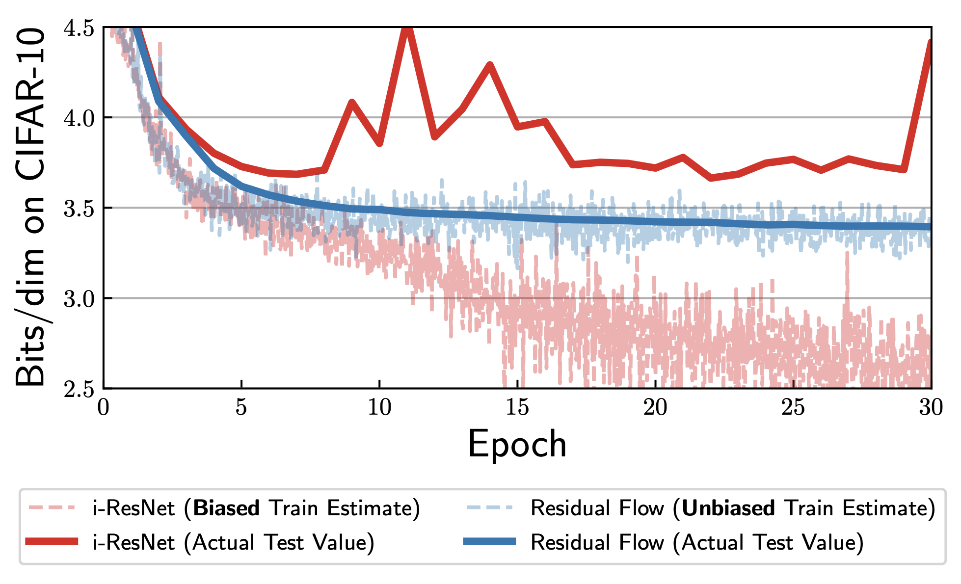
\[\mathbb{E}_{v}\left[v^T \left( \sum_{k=0}^{N} \frac{(-1)^k}{k\cancel{\mathbb{P}[N \ge k]}} J_g(x)^k\cancel{\mathbb{P}[N \ge k]} \right) v \right] = \mathbb{E}_{v}\left[v^T \left( \sum_{k=0}^{N} \frac{(-1)^k}{k} J_g(x)^k \right) v \right] = \text{Tr}\left( \sum_{k=0}^{N} \frac{(-1)^k}{k} J_g(x)^k \right).\]

Thus, the Roulette estimator is unbiased! This is the approach taken by the authors of [2]. The resulting approach (along with some other changes) amounts to an improved i-ResNet, and is given the name residual flow. They find that the bias of the non-Roulette estimator used by i-ResNet causes the model to learn to optimize the likelihood given by the truncated series rather than the full series. At inference time, the model performs worse than would be expected.

The i-ResNet optimizes a biased version of the true objective at training time, and performs considerably worse at inference time. The corresponding residual flow, which uses the Roulette estimator does not display this discrepancy. Figure taken from [2].

Implementing the Lipschitz Constraint

Up to this point, we’ve been making the assumption that our neural networks $g_\theta^i(x)$ have been had Lipschitz constant less than one. How do we actually accomplish this? The idea is that after every training iteration, after the weights $\theta$ have been updated, we need to “renormalize” $g_\theta^i(x)$. To ensure that $\text{Lip}(g_\theta^i)$ is at most some constant $c < 1$, we conservatively enforce the property that each linear layer of $g_\theta^i$ has Lipschitz constant at most one.

Recall that $g_\theta^i$ is the composition of some number of linear layers $W_j^i$ and some number of non-linearities $\varphi_j^i$ so that it looks something like

\[g_\theta^i = \varphi_2^i \circ W_2^i \circ \varphi_1^i \circ \circ W_1^i.\]

We will assume that the non-linearities $\varphi_j^i$ (having no trainable weights) have been chosen so as to guarantee the Lipschitz costraint already. The authors of [2] propose the LipSwish non-linearity which has desirable saturation properties (large second derivative) when the Lipschitz constant is high. To make sure that $\text{Lip}(W_j^i) \le c < 1$, after every optimization step we use power iteration and the Rayleigh quotient to approximate its Lipschitz constant $\tilde{\sigma}$ (recall that this is equivalent to computing the largest singular value), and then multiply $W_j^i$ by $\frac{c}{\sigma}$ if necessary (if $\sigma > c$).

Recall however that power iteration only yields a lower bound on the true value $\sigma$ of the largest singular value, so we cannot be completely sure that the resulting weight matrix has Lipschitz constant less than $c$. To the best of my understanding, this only occurs when the power iteration is initialized poorly (the projection of the initial vector onto the right-singular vector corresponding to the maximal singular value is zero), and that this poor initialization happens with probability zero if initialized randomly and appropriately. I could be mistaken though - feel free to let me know if the lower bound is due to some other reason.

Nevertheless, the authors of [1] find that in practice that this scheme works nearly perfectly, and that the resulting networks $g_\theta^i(x)$ have Lipschitz constant at most the value of the chosen $c$. Note here that conservatively enforcing the desired Lipschitz constraint on all layers as a means to indirectly enforce the same constraint on the map $g_\theta^i(x)$ could be limiting, and the authors admit that it might be a good idea to take a look into enforcing the property more directly.

Connections to Flow-Based Generative Models

Residual flows are discrete normalizing flows: they model the map $F_\theta$ as the discrete composition $F_\theta \triangleq F_\theta^N \circ \dots \circ F_\theta^1$. Recall that continuous normalizing flows parameterize via a time-dependent vector field $u_\theta(x,t)$. This is conceptually the same approach taken by diffusion models (more generally: score-based generative models), and, recently, with models trained with flow matching. We will use the term flow-based generative model as an umbrella term for these models.

If we imagine placing a particle at a point $(x,t)$, and letting the vector field transport the particle in time and space, we recover the “flow” of the vector field. Initial value problems, from ordinary differential equations, basically ask: if I start at $(x_0, t_0)$, and I “travel” or “flow” along the vector field for time $\Delta t$, where do I end up? Sampling from flow based generative models involves solving such a problem. With diffusion, for example, we sample $x_0$ from a Gaussian and set $t$ to be some arbitrarily large value, and then follow the probability flow ode to time $t=0$ at which point, if our model is perfect, we would have obtained a sample from the data distribution. In special cases, when the form of $u_\theta(x,t)$ is particularly simply, it is possible to find a closed-form answer to this question. In general, and especially when our vector field is parameterized as a neural network like $u_\theta(x,t)$ is, we must approximate the solution to this problem.

Now the big idea is that we can approximate a particle’s trajectory by repeatedly taking small steps in the direction of the vector field $u_\theta(x,t)$. This amounts to repeatedly making updates of the form

\[\begin{aligned} x &\to x + hu_\theta(x,t),\\ t & \to t + h. \end{aligned}\]

Here, $h$ is the step size. If we decrease our step size $h$, we approximate the true trajectory more faithfully (more accurate), but we must take more steps to travel a fixed distance in time (more expensive). Simple integrators like the one shown above are known as Euler integrators, and are the simplest of the much broader class of Runge-Kutta methods. The whole point is that these Euler integrators are effectively a residual flow with $g_\theta(x,t)$ given by

\[g_\theta^t(x) \triangleq hu_\theta(x,t),\]

provided that $\text{Lip}(u_\theta(x,t)) < 1$ (as a function of $x$). Thus, the capacity of residual flows to approximate various flow-based generative models comes down to the Lipschitz constants of their learned vector fields. For now, we will stop here.

Disclaimer: All mistakes and types are my own. If you think you’ve found one, please let me know and I’ll fix it.

References

[1] Jens Behrmann et al. Invertible Residual Networks. 2019. arXiv: 1811.00995 [cs.LG].

[2] Ricky T. Q. Chen et al. Residual Flows for Invertible Generative Modeling. 2020. arXiv: 1906.02735 [stat.ML]

[3] Haim Avron and Sivan Toledo. “Randomized algorithms for estimating the trace of an implicit symmetric positive semi-definite matrix”. In: Journal of the ACM (JACM) 58.2 (2011), pp. 1– 34.